imported>Andy |
imported>WikiSysop |
| Line 1: |
Line 1: |
| − | {{Navigation|Previous= [[The_Proof_Obligation_Explorer_(Rodin_User_Manual)|The Proof Obligation Explorer]]|Next= [[The_Mathematical_Language_(Rodin_User_Manual)|The Mathematical Language]]|Up= [[index_(Rodin_User_Manual)|User_Manual_index]]}}
| + | ==Modelling Structured Types== |
| − | {{TOCright}}
| |
| − | == Overview == | |
| − | When proof obligations (POs) are not discharged automatically the user can attempt to discharge them interactively using the Proving Perspective. This page provides an overview of the Proving Perspective and its use. If the Proving Perspective is not visible as a tab on the top right-hand corner of the main interface, the user can switch to it via "Window -> Open Perspective".
| |
| | | | |
| − | The Proving Perspective consists of a number of views: the Proof Tree, the Goal, the Selected Hypotheses, the Proof Control, the Search Hypotheses, the Cache Hypotheses and the Proof Information. In the discussion that follows we look at each of these views individually. Below is a screenshot of the Proving Perspective: | + | The Event-B mathematical language currently does not support a syntax for the direct definition of structured types such as records or class structures. |
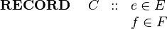
| | + | Nevertheless it is possible to model structured types using projection functions to represent the fields/attributes. For example, |
| | + | suppose we wish to model a record structure ''C'' with fields ''e'' and ''f'' (with type ''E'' and ''F'' respectively). |
| | + | Let us use the following syntax for this (not part of Event-B syntax): |
| | | | |
| − | [[Image:ProvPers.png|center]]
| + | <center> |
| | + | {{SimpleHeader}} |
| | + | |<math> \begin{array}{lcl} |
| | + | \textbf{RECORD}~~~~ C &::& e\in E\\ |
| | + | && f \in F |
| | + | \end{array} |
| | + | </math> |
| | + | |} |
| | + | </center> |
| | | | |
| − | == Loading a Proof ==
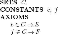
| + | We can model this structure in Event-B by introducing (in a context) a carrier set ''C'' and two |
| − | To work on an un-discharged PO it is necessary to load the proof into the Proving Perspective. To do this switch to the Proving Perspective; select the project from the Event-B Explorer; select and expand the component (context or machine); and finally select (double-click) the proof obligation of interest. A number of views will be updated with details of the corresponding proof.
| + | functions ''e'' and ''f'' as constants as follows: |
| − | [[Image:ExplorerView.png|center]]
| |
| | | | |
| − | == The Proof Tree ==
| + | <center> |
| − | The proof tree view provides a graphical representation of each individual proof step, as seen in the following screenshot:
| + | {{SimpleHeader}} |
| | + | |<math> \begin{array}{l} |
| | + | \textbf{SETS}~~ C\\ |
| | + | \textbf{CONSTANTS}~~ e,~ f\\ |
| | + | \textbf{AXIOMS}\\ |
| | + | ~~~~\begin{array}{l} |
| | + | e \in C \tfun E\\ |
| | + | f \in C \tfun F\\ |
| | + | \end{array} |
| | + | \end{array} |
| | + | </math> |
| | + | |} |
| | + | </center> |
| | | | |
| − | [[Image:ProTree.png|center]]
| |
| | | | |
| − | Each node in the tree corresponds to a sequent. A line is right shifted when the corresponding node is a direct descendant of the node of the previous line. Each node is labelled with a comment which indicates which rule has been applied, or which prover discharged the proof. By selecting a node in the proof tree, the corresponding sequent is loaded: the hypotheses of the sequent are loaded to the Selected Hypotheses window, and the goal of the sequent is loaded to the Goal view.
| + | Now, given an element <math>c\in C</math> representing a record structure, we write <math>e(c)</math> for the ''e'' component of ''c'' and <math>f(c)</math> for the ''f'' component of ''c''. |
| | | | |
| − | === Decoration===
| + | ''E'' and ''F'' can be any type definable in Event-B, including a type representing a record structure. |
| − | The leaves of the tree are decorated with one of three icons:
| |
| | | | |
| − | * [[Image:Discharged.gif]] means that this leaf is discharged,
| + | ==Constructing Structured Values== |
| − | * [[Image:Pending.gif]] means that this leaf is not discharged,
| |
| − | * [[Image:Reviewed.gif]] means that this leaf has been reviewed.
| |
| | | | |
| − | Internal nodes in the proof tree are decorated in reverse colours. Note that a "reviewed" leaf is one that is not discharged yet by the prover. Instead, it has been "seen" by the user who decided to postpone the proof. Marking nodes as "reviewed" is very convenient since the provers will ignore these leaves and focus on specific areas of interest. This allows interactive proof in a gradual fashion. In order to discharge a "reviewed" node, select it and prune the tree at that node: the node will become "brown" again (undischarged) and you can now try to discharge it.
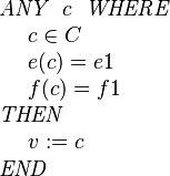
| + | Suppose we have a variable ''v'' in a machine whose type is the structure ''C'' defined above: |
| | + | <center> |
| | + | <math>\textit{VARIABLE}~~ v\in C</math> |
| | + | </center> |
| | + | We wish to assign a structured value to ''v'' whose ''e'' field has some value ''e1'' and whose ''f'' field has some value ''f1''. |
| | + | This can be achieved by specifying the choice of an event parameter ''c'' whose fields are constrained by appropriate guards |
| | + | and assigning parameter ''c'' to the machine variable ''v''. This is shown in the following event: |
| | | | |
| − | === Navigation within the Proof Tree=== | + | <center><math> |
| − | On top of the proof tree view, one can see three buttons:
| + | \begin{array}{l} |
| | + | \textit{ANY}~~ c ~~\textit{WHERE} \\ |
| | + | ~~~~ c \in C \\ |
| | + | ~~~~ e( c ) = e1 \\ |
| | + | ~~~~ f( c ) = f1 \\ |
| | + | \textit{THEN} \\ |
| | + | ~~~~ v := c \\ |
| | + | \textit{END} |
| | + | \end{array} |
| | + | </math></center> |
| | | | |
| − | * the "'''G'''" buttons allows you to see the goal of the sequent corresponding to each node,
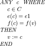
| + | If we only wish to update some fields and leave others changed, this needs to be done by specifying explicitly that some fields |
| − | * the "'''+'''" button allows you to fully expand the proof tree,
| + | remain unchanged. This is shown in the following example where only the ''e'' field is modified: |
| − | * the "'''-'''" allows you to fully collapse the tree: only the root stays visible.
| |
| | | | |
| − | === Manipulating the Proof Tree=== | + | <center><math> |
| | + | \begin{array}{l} |
| | + | \textit{ANY}~~ c ~~\textit{WHERE} \\ |
| | + | ~~~~ c \in C \\ |
| | + | ~~~~ e( c ) = e1 \\ |
| | + | ~~~~ f( c ) = f(v) \\ |
| | + | \textit{THEN} \\ |
| | + | ~~~~ v := c \\ |
| | + | \textit{END} |
| | + | \end{array} |
| | + | </math></center> |
| | | | |
| − | ==== Hiding ====
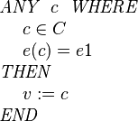
| + | If we don't care about the value of some field (e.g., ''f''), we simply omit any guard on that field as follows: |
| − | The little square (with a "+" or "-" inside) next to each node in the proof tree allows you to expand or collapse the subtree starting at that node.
| |
| | | | |
| − | ==== Pruning ==== | + | <center><math> |
| − | The proof tree can be pruned at a selected node; the subtree of the selected node is removed from the proof tree. The selected node becomes a leaf and is decorated with [[Image:Pending.gif]] . The proof activity can then be resumed from this node. After selecting a node in the proof tree pruning can be performed in two ways:
| + | \begin{array}{l} |
| − | * by right-clicking and then selecting "Prune",
| + | \textit{ANY}~~ c ~~\textit{WHERE} \\ |
| − | * by clicking the [[Image:Pn_prover.gif]] button in the proof control view.
| + | ~~~~ c \in C \\ |
| | + | ~~~~ e( c ) = e1 \\ |
| | + | \textit{THEN} \\ |
| | + | ~~~~ v := c \\ |
| | + | \textit{END} |
| | + | \end{array} |
| | + | </math></center> |
| | | | |
| − | Note that after pruning, the post-tactic is not applied to the new current sequent. The post-tactic should be applied manually, if required, by clicking the post-tactic button in the Proof Control view. This is useful, in particular, when you want to redo a proof from the beginning. The proof tree can be pruned at its root node and then the proof can proceed again, with invocation of internal or external provers; or with interactive proof.
| |
| | | | |
| − | Before pruning a particular node, the node (and its subtree) can be copied to the clipboard. If the new proof strategy subsequently fails, the copied version can be pasted back into the pruned node (see the next section).
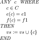
| + | Sometimes we will wish to model a set of structured elements as a machine variable, e.g., |
| | + | <center> |
| | + | <math>\textit{VARIABLE}~~ vs\subseteq C</math> |
| | + | </center> |
| | | | |
| − | ==== Copy/Paste ==== | + | We can add a structured element to this set using the following event: |
| | + | <center><math> |
| | + | \begin{array}{l} |
| | + | \textit{ANY}~~ c ~~\textit{WHERE} \\ |
| | + | ~~~~ c \in C \\ |
| | + | ~~~~ e( c ) = e1 \\ |
| | + | ~~~~ f( c ) = f1 \\ |
| | + | \textit{THEN} \\ |
| | + | ~~~~ vs := vs \cup \{c\} \\ |
| | + | \textit{END} |
| | + | \end{array} |
| | + | </math></center> |
| | | | |
| − | By selecting a node in the proof tree and then right-clicking with the mouse, you can copy the part of the proof tree starting at that sequent (the node and its subtree). Pasting the node and subtree back in is done in a similar manner, with a right mouse click on a proof node. This allows reuse of part of a proof tree in the same, or even in another, proof.
| + | ==Extending Structured Types== |
| | | | |
| − | == Goal and Selected Hypotheses == | + | ==Sub-Typing== |
| − | The nodes in the proof tree view correspond to sequents. A user will work with one selected node, and thus one sequent, at a time; attempting various strategies in an effort to show that the sequent goal is true. The "Goal" and "Selected Hypotheses" views provide information to the user about the currently selected sequent. Here is an example:
| |
| − | [[Image:GoalHyp.png|center]]
| |
| | | | |
| − | A hypothesis can be removed from the list of selected hypotheses by selecting the check the box situated next to it (you can click on several boxes) and then by clicking on the [[Image:remove.gif]] button at the top of the selected hypotheses window:
| + | ==Recursive Structured Types== |
| | | | |
| − | [[Image:GoalHypSelect.png|center]]
| + | ==Structured Variables== |
| − | | |
| − | Here is the result:
| |
| − | | |
| − | [[Image:GoalHypSelectRes.png|center]]
| |
| − | | |
| − | Note that the deselected hypotheses are not lost: you can find them again using the Search Hypotheses [[Image:sh_prover.gif]] button in the Proof Control view. Other buttons are used as follows:
| |
| − | | |
| − | | |
| − | * [[Image:select_all_prover.gif]] select all hypotheses.
| |
| − | | |
| − | | |
| − | * [[Image:inv_prover.gif]] invert the selection.
| |
| − | | |
| − | | |
| − | * [[Image:falsify_prover.gif]] next to the goal - proof by contradiction 1: The negation of the '''goal''' becomes a selected hypothesis and the goal becomes "'''⊥'''".
| |
| − | | |
| − | | |
| − | * [[Image:falsify_prover.gif]] next to a selected hypothesis - proof by contradiction 2: The negation of the '''hypothesis''' becomes the goal and the negated goal becomes a selected hypothesis.
| |
| − | | |
| − | | |
| − | === Applying Proof Rules === | |
| − | A user wishing to attempt an interactive proof has a number of proof rules available, and these may be either rewrite rules or inference rules. In the Goal and the Selected Hypotheses views various operators may appear in red coloured font. The red font indicates that some interactive proof rule(s) are applicable and may be applied as a step in the proof attempt. When the mouse hovers over such an operator a number of applicable rules may be displayed; the user may choose to apply one of the rules by clicking on it.
| |
| − | | |
| − | Other proof rules can be applied when green buttons appear in the Goal and Selected Hypotheses views. Examples are proof by contradiction [[Image:falsify_prover.gif]], that we have already encountered; and [[Image:ConjI_prover.gif]] for conjunction introduction in the goal.
| |
| − | | |
| − | [[Image:ApplyRewRule.png|center]]
| |
| − | | |
| − | ==== Rewrite Rules ====
| |
| − | Rewrite rules are one-directional equalities (and equivalences) that can be used to simplify formulas (the goal or a single hypothesis). A rewrite rule is applied from left to right when its ''side condition'' holds; it can be applied either in the goal predicate, or in one of the selected hypotheses.
| |
| − | | |
| − | A rewrite rule is applied either automatically ('''A''') or manually ('''M'''):
| |
| − | * automatically, when post-tactics are run.
| |
| − | * automatically, when auto-tactics are run.
| |
| − | * manually, through an interactive command. These rules gather non equivalence laws, definition laws, distributivity laws and derived laws.
| |
| − | | |
| − | Automatic rewrite rules are equivalence simplification laws.
| |
| − | | |
| − | Each rule name indicates the rule's characteristics according to the following convention:
| |
| − | | |
| − | * the law category: simplification law (SIMP), definition law (DEF), distributivity law (DISTRI), or else derived law (DERIV).
| |
| − | * the root operator of the formula on the left-hand side of the rule, e.g. predicate AND, expression BUNION.
| |
| − | * (optionally) the terminal elements on the left-hand side of the rule: special element (SPECIAL) such as the empty-set, type expression (TYPE), same element occurring more than once (MULTI), literal (LIT). A type expression is either a basic type (<math>\intg, \Bool</math>, any carrier set), or <math>\pow</math>(type expression), or type expression<math>\cprod</math>type expression.
| |
| − | * (optionally) some other description of a characteristic, e.g. left (L), right (R).
| |
| − | | |
| − | Rewrite rules having an equivalence operator on the left-hand side may also describe other rules. eg: the rule:
| |
| − | | |
| − | <center><math> \True = \False \;\;\defi\;\; \bfalse </math></center>
| |
| − | | |
| − | should also produce the rule:
| |
| − | | |
| − | <center><math> \False = \True \;\;\defi\;\; \bfalse </math></center>
| |
| − | | |
| − | For associative operators in connection with distributive laws as in:
| |
| − | | |
| − | <center><math> P \land (Q~ {\color{red}{\lor}} \ldots \lor R) </math></center>
| |
| − | | |
| − | it has been decided to highlight the first associative/commutative operator (the <math>{\color{red}{\lor}} </math>). A menu is presented when hovering the mouse over the operator: the first menu option distributes all associative/commutative operators, the second option distributes only the first associative/commutative operator. In order to simplify the explanation we write associative/commutative operators with two parameters only. However, ''we must emphasise here'', that generally we may have a sequence of more than two parameters. So, we write <math> Q \lor R </math> instead of <math> Q \lor \ldots \lor R </math>. Rules are sorted according to their purpose.
| |
| − | | |
| − | Rules marked with a star in the first column are implemented in the current prover. Rules without a star are planned for implementation.
| |
| − | | |
| − | Rewrite rules are split into:
| |
| − | | |
| − | * [[Set Rewrite Rules]]
| |
| − | * [[Relation Rewrite Rules]]
| |
| − | * [[Arithmetic Rewrite Rules]]
| |
| − | | |
| − | They are also available in a single large page [[All Rewrite Rules]].
| |
| − | | |
| − | ==== Inference Rules ====
| |
| − | Inference rules (see [[Proof Rules]]) are applied either automatically (A) or manually (M).
| |
| − | | |
| − | Inference rules applied automatically are applied at the end of each proof step. They have the following possible effects:
| |
| − | | |
| − | * they discharge the goal,
| |
| − | * they simplify the goal and add a selected hypothesis,
| |
| − | * they simplify the goal by decomposing it into several simpler goals,
| |
| − | * they simplify a selected hypothesis,
| |
| − | * they simplify a selected hypothesis by decomposing it into several simpler selected hypotheses.
| |
| − | | |
| − | Inference rules applied manually are used to perform an interactive proof. They can be invoked by clicking the red highlighted operators in the goal or the hypotheses. A menu is presented when there are several options.
| |
| − | | |
| − | See [[Inference Rules]] list.
| |
| − | | |
| − | == The Proof Control View==
| |
| − | | |
| − | The Proof Control view contains the buttons which you can use to perform an interactive proof.
| |
| − | | |
| − | [[Image:PControl.png|center]]
| |
| − | | |
| − | The Proof Control view offers a number of buttons whose effects we briefly describe next; moving from left to right on the toolbar:
| |
| − | | |
| − | * ('''nPP''') invokes the new predicate prover, a drop-down list indicates alternative strategies.
| |
| − | * ('''R''') indicates that a node has been reviewed: in an attempt by the user to carry out proofs in a stepwise fashion, they might decide to postpone the task of discharging some proofs until a later stage. To do this the proofs can be marked as reviewed by choosing the proof node and clicking this button. This indicates that by visually checking the proof the user is convinced that they can discharge it later, but they do not want to do it right now.
| |
| − | * ('''p0''') the PP and ML provers can be invoked from the drop-down list using different forces.
| |
| − | * ('''dc''') do proof by cases: the proof is split into two branches. In the first branch:- the predicate supplied by the user is added to the Selected Hypotheses, and the user attempts to discharge this branch. In the second branch :- the predicate supplied by the user is negated and added to the Selected Hypotheses; the user then attempts to discharge this branch.
| |
| − | | |
| − | * ('''ah''') add a new lemma: the predicate in the editing area should be proved by the user. It is then added as a new selected hypothesis.
| |
| − | * ('''ae''') abstract expression: the expression in the editing area is given a fresh name.
| |
| − | * '''the robot''': invokes the auto-prover which attempts to discharge the goal. The auto-prover is applied automatically on all proof obligations after a "save" without any intervention of the user. Using this button, you can invoke the auto-prover within an interactive proof.
| |
| − | * the '''post-tactic''' is executed ,
| |
| − | * '''lasoo''': load into the Selected Hypotheses window those hidden hypotheses that contain identifiers in common with the goal, and with the selected hypotheses.
| |
| − | * '''backtrack''' form the current node (i.e., prune its parent),
| |
| − | * '''scissors''': prune the proof tree from the node selected in the proof tree,
| |
| − | * '''Search Hypotheses''': find hypotheses containing the character string in the editing area, and display in the Search Hypothesis view.
| |
| − | * '''Cache Hypotheses''': press this to display the ''"Cache Hypotheses"'' view. This view displays all hypotheses that are related to the current goal.
| |
| − | * load the '''previous''' undischarged proof obligation,
| |
| − | * load the '''next''' undischarged proof obligation,
| |
| − | * '''(i)''' show information corresponding to the current proof obligation in the corresponding window. This information correspond to the elements that directly took part in the proof obligation generation (events, invariant, etc.),
| |
| − | * goto the next '''pending''' node of the current proof tree,
| |
| − | * load the next '''reviewed''' node of the current proof tree.
| |
| − | * '''Disable/Enable Post-tactics''': allows the user to choose whether post-tactics run after each interactive proof step.
| |
| − | === The Smiley ===
| |
| − | The smiley can be one of three different colors: (1) red, indicates that the proof tree contains one or more undischarged sequents, (2) blue, indicates that all undischarged sequents of the proof tree have been reviewed, (3) green, indicates that all sequents of the proof tree are discharged.
| |
| − | | |
| − | === The Editing Area ===
| |
| − | The editing area allows the user to supply parameters for proof commands. For example, when the user attempts to add a new hypothesis (by clicking the lemma '''ah''' button), the new hypothesis should have been written by the user in the editing area.
| |
| − | | |
| − | === ML/PP and Hypotheses ===
| |
| − | | |
| − | ==== ML ====
| |
| − | ML (mono-lemma) prover appears in the drop-down list under the button ('''pp''') as M0, M1, M2, M3, ML.
| |
| − | The different configuration (e.g., M0) refer to the proof force of the ML prover. '''All hypotheses''' are passed to ML.
| |
| − | | |
| − | ==== PP ====
| |
| − | PP (predicate prover) appears in the drop-down list under the button ('''pp''') as P0, P1, PP.
| |
| − | * P0 uses '''all selected hypotheses''' (the ones in '''Selected Hypotheses''' window).
| |
| − | * P1 employs a '''lasoo''' operation to the selected hypotheses and the goal, and uses the resulting hypotheses.
| |
| − | * PP uses '''all hypotheses'''.
| |
| − | | |
| − | == The Search Hypotheses View==
| |
| − | | |
| − | By typing a string in the editing area of the Proof Control window and pressing the Search Hypotheses button, a window is displayed which contains the hypotheses matching a character string provided by the user in the editing area.
| |
| − | | |
| − | [[Image:SearchHyp.png|center]]
| |
| − | | |
| − | To move any of these hypotheses to the '''Selected Hypotheses''' window, select those required (using the check boxes) and press the [[Image:Add.gif]] button. Adding these hypotheses to the selected hypotheses means that they will be visible to the prover. They can then be used during the next interactive proof phase.
| |
| − | | |
| − | To remove hypotheses from the '''Search Hypotheses''' window use the [[Image:Remove.gif]] button. This button also appears above the selected hypotheses, and allows the user to remove any hypothesis from the '''Selected Hypotheses''' window.
| |
| − | | |
| − | The other button, situated to the left each hypotheses, is the [[Image:falsify_prover.gif]] button. Pressing this will attempt a proof by contradiction. The effect is the same as if the hypothesis were in the '''Selected Hypotheses'''.
| |
| − | | |
| − | == The Cache Hypotheses Window ==
| |
| − | | |
| − | This window allows the user to keep track of recently manipulated (e.g., used, removed, selected) hypotheses for any PO. For example, when the user applies a rewrite to an hypothesis, a new hypothesis (after the rewriting) is selected, and the original hypothesis is deselected and put in the '''Cache Hypotheses''' window.
| |
| − | | |
| − | Similar operations (to that of the '''Selected Hypotheses''' and '''Search Hypotheses''' windows) such as removing, selecting and proof by contradiction ('''ct''') are also available for the cached hypotheses. Interactive proof steps (e.g., rewriting) can also be carried out from the '''Cache Hypotheses''' window as well as the '''Search Hypotheses''' window.
| |
| − | | |
| − | == Proof Information View ==
| |
| − | | |
| − | This view displays information so that the user can relate a proof obligation to the model. For example, typical information for an event invariant preservation PO includes the event; as well as the invariant in question.
| |
| − | | |
| − | [[Image:PInfo.png|center]]
| |
| − | | |
| − | == Auto-tactic and Post-tactic ==
| |
| − | | |
| − | The auto-tactic applies a combination of ''rewrite'', ''inference'' and ''external provers'' to newly generated proof obligations. However, they can also be invoked by the user by clicking on the [[Image:auto_prover.png]] button in the '''Proof Control''' view.
| |
| − | | |
| − | Post-tactic is also a combination of ''rewrite'', ''inference'' and ''external provers'', and is applied automatically after each interactive proof step. However, it can also be invoked manually by clicking on the [[Image:Broom_prover.gif]] button in the '''Proof Control''' view. Note that the post-tactic can be disabled by clicking the [[Image:disable_xp_prover.gif]] button, situated on the right of the '''Proof Control''' view.
| |
| − | | |
| − | === Preferences for the Auto-tactic ===
| |
| − | | |
| − | The auto-tactic can be configured by means of a preference page which can be found as follows: Click on "Window" in the top toolbar; in the drop-down menu select "Preferences". Expand the "Event-B" option from the list; then "Sequent Prover", and finally select "Auto-Tactic". The following window is displayed:
| |
| − | | |
| − | [[Image:AutoTac.png|center]]
| |
| − | | |
| − | A list of available tactics appear in the left-hand box. A list of tactics selected for inclusion by the auto-tactic appears in the right-hand box. By selecting a tactic, in either list, it can be moved from one list to another. By clicking on a tactic in the right-hand list it may be moved up or down, since the order of tactic application is determined by the order of this list.
| |
| − | | |
| − | === Preferences for the Post-tactic ===
| |
| − | | |
| − | The post-tactic can be configured by navigating to the same menu that includes the auto-tactic preferences and then selecting "Post-Tactic". The preferences are selected in the same way as the auto-tactic. The following window is displayed:
| |
| − | | |
| − | [[Image:PostTac.png|center]]
| |
| − | | |
| − | [[Category:User documentation|The Proving Perspective]]
| |
| − | [[Category:Rodin Platform|The Proving Perspective]]
| |
| − | [[Category:User manual|The Proving Perspective]]
| |
 representing a record structure, we write
  for the e component of c and
  for the f component of c.